We have carried out in this project two types of experiments involving the collapse of different visco-plastic materials (sand and liquid soap) on non-planar bottom surfaces.  The laboratory tests were used in tuning the coefficients (viscosity, internal friction coefficient and cohesion) of the mechanical model such that the whole model (depth-averaged mechanical model and its numerical approach) fits well with the experiment.

  1) Two-dimensional tests

  The first experimental set up was designed for a two dimensional comparison between the experiment and the depth-averaged model. The experimental setup consists of a narrow channel between Plexiglas walls with a spacing of 10 cm (see Figure 1).  Three geometries of the bottom geometries where considered (See Figure 1) but the reservoirs dimensions (0.20x0.30x0.10) were the same for all these three geometries. The reservoir has a door, which opens in the experimental plane, such that the entire fluid column is liberated at once. This point is important in Saint-Venant modeling, where we deal with depth-integrated models, which cannot describe a time evolution of the door in the vertical plane.  The non-planar channel is 1m long. A rectangular granular mass of thickness 20 cm is released from a reservoir by opening the gate. The visco-plastic material flows down on the channel with a Plexiglas bottom surface. The length of the deposit is measured and the final thickness of the deposit at the back wall will be systematically recorded as well as the time at which the front stopped. The profiles of the granular mass have been recorded using a high-speed (1000fps) camera.

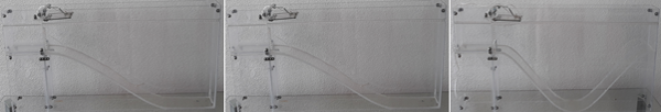
Figure 1: Three configurations of the 2-D experiment.

  Dry sand. The first material that has been tested was the dry sand.   The grain size distribution in the sand was fine to medium, with a grain size around 0.5mm and a density of 1450 kg/m3.  In Fig 2 we have plotted two snapshots of the experiment and we have compared them with a “tuned” numerical model.  The parameters for sand that we have found are:  fluid viscosity=1Pas, cohesion= 1Pa, internal frictional angle=30°, bottom frictional angle= 25° and bottom frictional viscosity=0.1Pas/m, which very close to the real physical parameters. We remark a good agreement between the « tuned » computational model and the experiment.

  Liquid Soap. The second material that we have tested was the liquid soap. We have chosen this material for its properties in modeling the mud or the lava.  The measured density of the liquid soap was 1050 kg/m3.  In Fig 2 we have plotted two snapshots of the experiment and we have compared them with a “tuned” numerical model.  The parameters for sand that we have found are:  fluid viscosity=10 Pas, yield stress = 25Pa, internal frictional angle =0°, bottom frictional angle  = 3°, and bottom frictional viscosity =5Pas/m.  As for the sand flowing we remark a good agreement between the « tuned » computational model and the experiment.

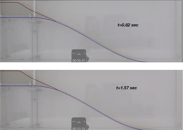
 Figure 2: Two snapshots of sand flowing in a narrow channel between Plexiglas walls: numerical simulation (in red line) versus the experiment (photo).

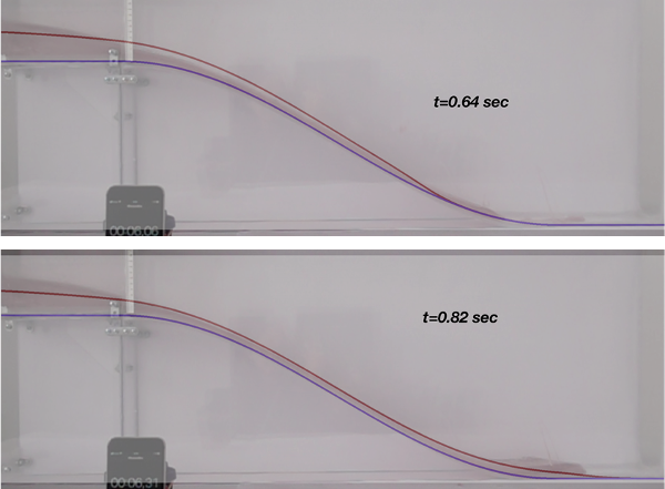
 Figure 3: Two snapshots of liquid soap flowing in a narrow channel between Plexiglas: numerical simulation (in red line) versus the experiment (photo).

  2) Three-dimensional tests

  The second type of experiment concerns the flow from a reservoir, after a dam breaking, over a bottom with a three dimensional topography given by an analytical function.
The experimental device has a reservoir (see Figure 4) with a door, which opens in the Ox1x2 plane for modeling the dam break, such that all the fluid in front of the door is liberated at once. As for the two-dimensional experiment, this point is important. Indeed, in the Saint-Venant approach, which is a thickness integrated model, we cannot describe a time evolution of the door in the vertical plane.  Since the geometrical description of the fluid domain is related to the normal vector at the bottom, the shape of the door (i.e. the part of the dam which was broken), which has to be described from the normal direction on the bottom, was chosen to fulfill this specific description.

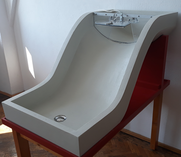
  Figure 4: The three dimensional experiment for modeling the flow from a reservoir after a dam break over a bottom with topography.

  Dry sand. The first material that has been tested in this experiment was the dry sand. The parameters for sand that we have been used in the computations were found (“tuned”) in the previous two-dimensional tests (i.e. density=1450 kg/m3, fluid viscosity=1Pas, cohesion= 1Pa, internal frictional angle=30°, bottom frictional angle= 25° and bottom frictional viscosity=0.1Pas/m). In Figure 5 we have plotted four snapshots of the experiment and we have compared them with a “tuned” numerical model. We remark a good agreement between the « tuned » computational model and the experiment.

  Liquid Soap. The second material that has been tested in the 3-D experiment was the liquid soap. The parameters that we have been used in the computations were found (“tuned”) in the previous two-dimensional tests (i.e. density=1050 kg/m3, fluid viscosity=10 Pas, yield stress = 25Pa, internal frictional angle =0°, bottom frictional angle  = 3°, and bottom frictional viscosity =5Pas/m). In Figure 6 we have plotted four snapshots of the experiment and we have compared them with a “tuned” numerical model. As for the dry sand we remark a good agreement between the « tuned » computational model and the experiment.

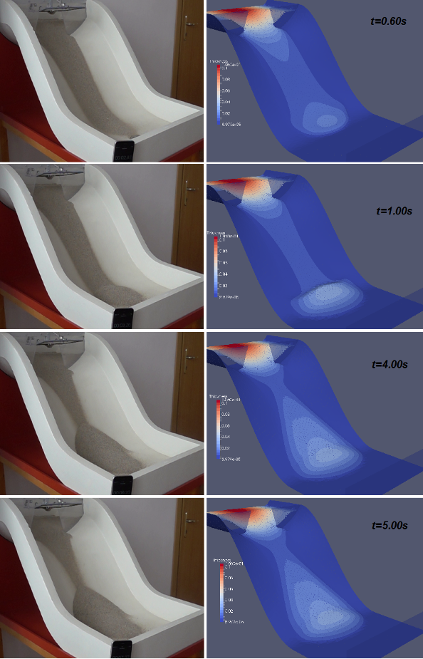
 Figure 5: Four snapshots of dry sand  flowing from a reservoir after a dam breaking over a bottom with a three dimensional  topography: numerical simulation (right) versus the experiment (left).

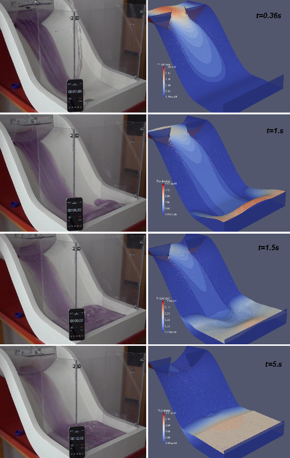
  Figure 6: Four snapshots of liquid soap  flowing from a reservoir after a dam breaking over a bottom with a three dimensional  topography: numerical simulation (right) versus the experiment (left).