This working package focused on the several software, implemented in C++,  for a  user-friendly  online use of the numerical programs and of the mechanical model. It illustrates the nowadays-successful transfer method of the scientific research results to the users via specialized software. This software will permit to a user to have a free computation of the flow over a topography for a large class of geophysical fluids and geophysical scenarios. The user-friendly software was constructed starting from the FreeFem++ code, which was already constructed (see sections 3.1 and 3.2) for the validation of the numerical approach.

  Let us describe here the user-friendly approach of the online use of the numerical scheeme. First of all the user have to arrive on to www.dales.csm.ro and create an account (name, email address, institution), which have to be validated by the Dales’ webmaster, and download the freeware Parawiew from https://www.paraview.org/download/. The general plan of the user-friendly software designed to compute geophysical flows over topography, can be found in Figure 2. It has 5 mandatory steps and two optional steps.

  Step 1: Topography. The first step consists in uploading the topography as a text file. The file contains the topography as a (vertical) elevation  Z(X,Y)  on a uniform grid on the XY-plane.  The user has to give the grid spacing size (say for instance s) and the name of the considered topography (say for instance T).  The user output of this step will be the file “T.vtk”  which have be downloaded on his computer and visualized with  Paraview. A typical topography view is plotted in Figure 1 and represents the east part of Almaj Mountains in Romanian Carpathians. If the user is satisfied of the result then this step is finished, if not he has to restart it.  There are two internal outputs of the this step the files “T.data” and “T.msh” where the server will record general information of the topography and of the generated mesh.

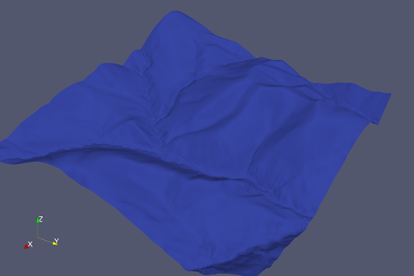
Figure 1: A typical topography view (representing the east part of Almaj mountains in Romanian Carpathians) of the end of Step 1.

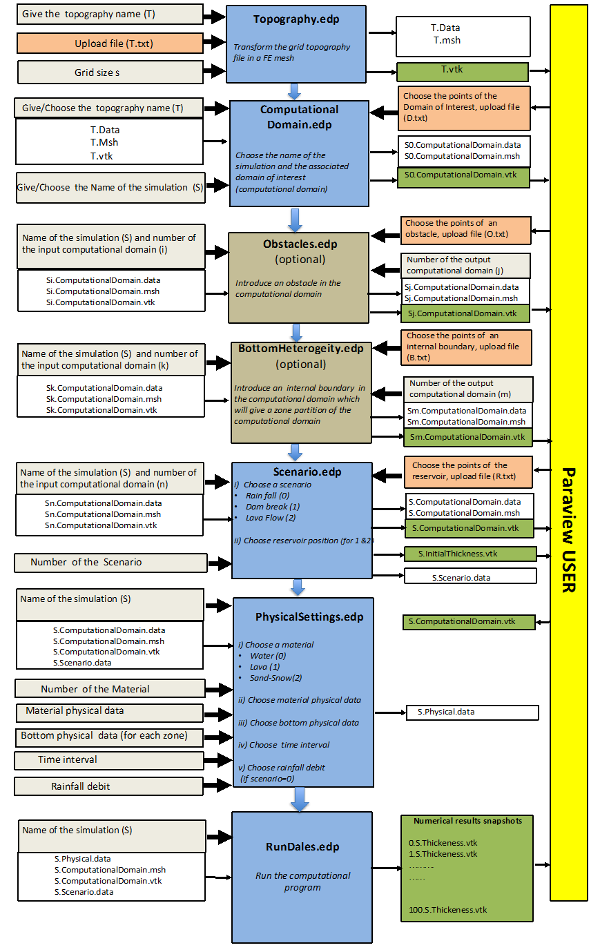Figure 2: The general plan of the user-friendly software to compute geophysical flows over a topography.

  Step 2: Computational Domain. The second step is focused on the definition of the computational (or interest) domain associated to a simulation.  First, the user has to choose the name of a topography (T), which was already uploaded at step 1, and to give a name for the numerical simulation he wants to run (say S).  Then the user has to go into the Paraview image and to choose the vertexes of a polygonal domain. The Paraview program will give him the positions of these points, which have to be copy-pasted in a text file (.txt ) and uploaded on the Dales server. All this procedure is explained in a tutorial, which will be available on the Dales website.  A typical example of this tutorial is plotted in Figure 3.

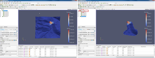
 Figure 3: An example of the tutorial used in the interpaly between the Dales server and the user’s Paraview session.

  At the end of Step 2, the output is file “S0.ComputationalDomain.vtk”, which have be downloaded on his computer and visualized with Paraview. A typical computational domain view is plotted in Figure 4.  If the user is satisfied of the result then this step is finished, if not he has to restart it.

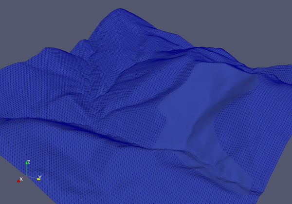
 Figure 4: A typical computational domain view at the end of Step 2.

  There are two internal outputs of the this step the files “S0.CoputationalDomain.data” and “S0.ComputationalDomain.msh” where the server will record general information of the computational and of the generated mesh.

  Step 2.1 (optional). Including obstacles. In this optional step the user can introduce obstacles, as polygonal domains, which will be considered outside the computational domain. The output is a new computational domain (say “S1.ComputationalDomain.vtk”), which have be downloaded on his computer and visualized with Paraview. A typical computational domain view is plotted in Figure 5. If the user is satisfied of the result then this step is finished, if not he has to restart it.

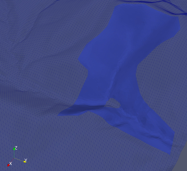
 Figure 5: A typical view of the computational domain with an obstacle at the end of Step 2.1.

  As before, there are two internal outputs of this step, the files “S1.CoputationalDomain.data” and “S1.ComputationalDomain.msh” where the server records general information of the computational domain and of the generated mesh.

  Step 2.2 (optional). Including bottom heterogeneity.  In this optional step the user can introduce different zones in the computational bottom domain, which have different resistance properties on the flow of a geophysical fluid.  The output is a new computational domain (say “S3.ComputationalDomain.vtk”), which have be downloaded on his computer and visualized with Paraview. A typical computational domain view is plotted in Figure 6. If the user is satisfied of the result then this step is finished, if not he has to restart it.  As before, there are two internal outputs of this step the files “S3.CoputationalDomain.data” and “S3.ComputationalDomain.msh” where the server will record general information of the computational and of the generated mesh.

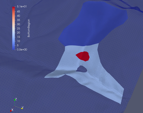
 Figure 6: A typical view of the computational domain with an obstacle and three bottom resistance regions at the end of Step 2.2.

  Step 3: Scenario choice. In this mandatory step the user have to choose the geophysical scenario. He has three choices: Rainfall, Dam break or Lava Flow. If the second, or the third case, the user have to choose the reservoir domain. To do that he have to go into the Paraview session and to choose the vertexes of a  polygonal domain in the computational domain. The Paraview program will give him the positions of these points, which have to be copy-pasted in a text file (.txt ) and uploaded on the Dales server. At the end of Step 3, the outputs are files “S.ComputationalDomain.vtk”  and “S.InitialThickness.vtk”,  which have be downloaded on his computer and visualized with Paraview. A typical computational domain view is plotted in Figure 7. If the user is satisfied of the result then this step is finished, if not he has to restart it.

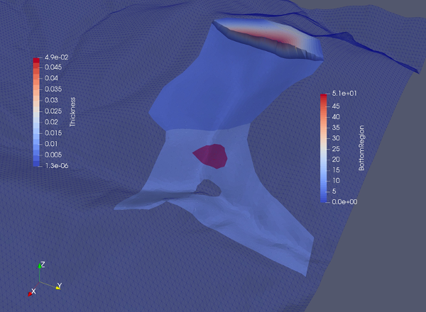
 Figure 7: A typical view of the computational domain and of the initial thickness in a dam-break scenario at the end of Step 3.

There are several internal outputs of this step the files. “S.CoputationalDomain.data” and “S.ComputationalDomain.msh” record general information of the computational doamin and of the generated mesh.  The file “S.Scenario.data” records the scenario choice of the simulation S.

  Step 4: Physical data. Here the user will have to choose the material settings. First he have to choose between three types of materials i) Water-type (i.e. incompressible Navier-Stokes fluid), ii) Lava-type (i.e. Bingham fluid) or iii) Sand-Snow-type (i.e. incompressible Drucker-Prager pressure dependent fluid). After that he have to give the material data for his choice (viscosity, yield limit for lava-type, cohesion and internal frictional angle for sand-snow type) or to use the values setted by the Dales-server.  After that the user have to choose the bottom physical data. Has has to give on each bottom region the resistance parameters: the turbulent frictional for water-type material of the bottom frictional coefficient and frictional viscosity for lava-type or sand-snow type materials.   After this setting the user is asked to give the length of time interval. Finally, in the case of rainfall scenario the user is asked to give the rainfall debit and the time length of the rainfall.  The output of this step is the file “S.Physical.data”, were all the information on the material settings is recorded.

  Step 5: Runing the program. In this step the user will start the computation of his simulation S. The inputs are the files “S.Physical.data”, “S.Scenario.data”, “S.CoputationalDomain.data”, “S.ComputationalDomain.msh” and “S.InitialThickness.vtk”. The final outputs of the simulation S are 100 snapshots of the computed flow, represented by the files “0.S.Thickness.vtk”, “1.S.Thickness.vtk”,... “100.S.Thickness.vtk”, which have be downloaded on his computer and visualized with Paraview. A typical view of the flow evolution is plotted in Figure 8.

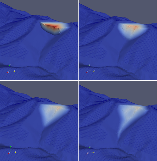
  Figure 8: Four snapshots of the computed flow evolution in a dam-break scenario for sand at the end of Step 5.